Google Data Analytics Professional Certificate

Capstone #1 - Bellabeat

Andrew Benjamin
June 4, 2022

library(ggplot2)
library(dplyr)
library(tidyverse)

Brief Introduction
Step 1 - Ask
- Business Task
Step 2 - Prepare
- Description of Data Sources
Step 3 - Process
Documented Cleaning Process
Step 4 - Analyze
- Summary of Analysis
Step 5 - Share
- Visualizations and Key Findings
Step 6 - Act
- Insights and Recommendations

Brief Introduction

In this project I am working as a Marketing Analyst for a company named Bellabeat, a high-tech manufacturer of health-focused products for women. The data set my stakeholder, Sršen, has provided me represents smart device users who are not using Bellabeat products. My job is to draw insights from this data and answer the questions below.

Step 1 - Ask

Sršen asks you to analyze smart device usage data in order to gain insight into how consumers use non-Bellabeat smart devices. She then wants you to select one Bellabeat product to apply these insights to in your presentation. These questions will guide your analysis:

What are some trends in smart device usage? Consumers use their smart devices in a variety of ways including to track sleep, measure intensity of activity, and to log weight information.
How could these trends apply to Bellabeat customers? The way non Bellabeat smart device users use their smart devices will likely resemble that of Bellabeat users. Thus analyzing these trends will allow the marketing team to better understand potential Bellabeat customers.
How could these trends help influence Bellabeat marketing strategy? These trends will pinpoint the usage of smart devices and help focus marketing those strengths to future Bellabeat customers.

Guiding questions

What is the problem you are trying to solve? Understanding insights from data in order to better inform marketing strategy for the Bellabeat app.
How can your insights drive business decisions? The insights from these data sets can help drive business decisions because they represent important business insights like how people use their products, demographic, and time stamps.

Business Task

Bellabeat has hired a team of data analysts to analyze smart device usage data in order to gain insight into how consumers are using non-Bellabeat smart devices. The trends I discover in this data set will help influence the marketing strategy for the Bellabeat app.

Step 2 - Prepare

Where is your data stored? My data is stored in Excel.
How is the data organized? Is it in long or wide format? My data is organized in long format.
Are there issues with bias or credibility in this data? Yes there are issues with bias and credibility because it is a survey. The bias comes to play becasuse only users who are interested in responding provide the data. Secondly, the amount of data provided is from 30 users which is not a large enough sample size for credible data. Lastly, there are outside factors which could affect data results. For example: time line, the data supplied is for 2 months in the spring, however, exercise habits change from season to season which may affect trends in data source.
Does your data ROCCC? The data is reliable and is from a trustworthy source. The data is original because it comes from 30 original users. The data is not comprehensive due to low sample size. The data is not current rather it is relatively old (2016). The data is cited from Amazon Mechanical Turk.
How are you addressing licensing, privacy, security, and accessibility? There are no licensing or privacy issues because data comes from an open source, security is fine because no personal information is used, and accessibility is open.
How did you verify the data’s integrity? In order to mantain integrity logs of manipulation were maintained and data was kept in one secure location.
How does it help you answer your question? We can use the data from smart device users to help understand trends in usage and influence the marketing strategy of the Bellabeat app.
Are there any problems with the data? Yes, in this data set there is missing data, outliers, and light formatting issues.

Description of Data Sources

FitBit Fitness Tracker Data (CC0: Public Domain, dataset made available through Mobius): This Kaggle data set contains personal fitness tracker from thirty fitbit users. Thirty eligible Fitbit users consented to the submission of personal tracker data, including minute-level output for physical activity, heart rate, and sleep monitoring. It includes information about daily activity, steps, and heart rate that can be used to explore users’ habits.

Step 3 - Process

What tools are you choosing and why? I chose Excel and R for data cleaning and visualizations and tableau for a dashboard.
Have you ensured your data’s integrity? Yes, throughout my process I logged updates and changes to these data sets.
What steps have you taken to ensure that your data is clean? In order to ensure that my data is clean I checked formatting, blank cells, white spaces, misspellings, and duplicates.
How can you verify that your data is clean and ready to analyze? I verified that my data was clean and ready to analyze by ensuring that the formatting was correct. I removed and updated missing data and checked for misspellings.
Have you documented your cleaning process so you can review and share those results? Yes, see next section.

Documented Cleaning Process

Import datasets

First I import sleepDay_merged, weightLogInfo_merged, heartrate_seconds_merged, and hourlyIntensities data sets.

sleep_data <- read.csv("/cloud/project/capstone project/R Projects/sleepDay_merged.csv")

weightLog_data <- read.csv("/cloud/project/capstone project/R Projects/weightLogInfo_merged.csv")

heartrate_data <- read.csv("/cloud/project/capstone project/R Projects/heartrate_seconds_merged.csv")

hourlyIntensities_data <- read.csv("/cloud/project/capstone project/R Projects/hourlyIntensities_merged.csv")

View datasets

Next, I viewed the heads of these data sets

glimpse(sleep_data)

## Rows: 419
## Columns: 10
## $ Id                 <dbl> 1503960366, 1503960366, 1503960366, 1503960366, 150…
## $ SleepDay           <chr> "Tuesday, April 12, 2016", "Wednesday, April 13, 20…
## $ TotalSleepRecords  <int> 1, 2, 1, 2, 1, 1, 1, 1, 1, 1, 1, 1, 1, 1, 1, 1, 1, …
## $ TotalMinutesAsleep <dbl> 327, 384, 412, 340, 700, 304, 360, 325, 361, 430, 2…
## $ TotalTimeInBed     <dbl> 346, 407, 442, 367, 712, 320, 377, 364, 384, 449, 3…
## $ Total.hours.asleep <int> 5, 6, 7, 6, 12, 5, 6, 5, 6, 7, 5, 4, 6, 6, 7, 6, 5,…
## $ Total.hours.in.bed <int> 6, 7, 7, 6, 12, 5, 6, 6, 6, 7, 5, 5, 7, 6, 7, 7, 5,…
## $ subtraction        <int> 0, 0, 1, 0, 0, 0, 0, 1, 0, 0, 1, 0, 0, 0, 0, 0, 1, …
## $ differenceminutes  <int> 19, 23, 30, 27, 12, 16, 17, 39, 23, 19, 46, 29, 27,…
## $ X                  <chr> "", "", "", "", "", "", "", "", "", "", "", "", "",…

glimpse(weightLog_data)

## Rows: 67
## Columns: 8
## $ Id             <dbl> 1503960366, 1503960366, 1927972279, 2873212765, 2873212…
## $ Date           <chr> "5/2/2016 23:59", "5/3/2016 23:59", "4/13/2016 1:08", "…
## $ WeightKg       <dbl> 52.6, 52.6, 133.5, 56.7, 57.3, 72.4, 72.3, 69.7, 70.3, …
## $ WeightPounds   <dbl> 115.9631, 115.9631, 294.3171, 125.0021, 126.3249, 159.6…
## $ Fat            <int> 22, NA, NA, NA, NA, 25, NA, NA, NA, NA, NA, NA, NA, NA,…
## $ BMI            <dbl> 22.65, 22.65, 47.54, 21.45, 21.69, 27.45, 27.38, 27.25,…
## $ IsManualReport <lgl> TRUE, TRUE, FALSE, TRUE, TRUE, TRUE, TRUE, TRUE, TRUE, …
## $ LogId          <dbl> 1.46e+12, 1.46e+12, 1.46e+12, 1.46e+12, 1.46e+12, 1.46e…

glimpse(heartrate_data)

## Rows: 1,048,575
## Columns: 5
## $ Id    <dbl> 2022484408, 2022484408, 2022484408, 2022484408, 2022484408, 2022…
## $ Time  <chr> "7:21 AM", "7:21 AM", "7:21 AM", "7:21 AM", "7:21 AM", "7:22 AM"…
## $ Value <int> 97, 102, 105, 103, 101, 95, 91, 93, 94, 93, 92, 89, 83, 61, 60, …
## $ X     <lgl> NA, NA, NA, NA, NA, NA, NA, NA, NA, NA, NA, NA, NA, NA, NA, NA, …
## $ X25   <lgl> NA, NA, NA, NA, NA, NA, NA, NA, NA, NA, NA, NA, NA, NA, NA, NA, …

glimpse(hourlyIntensities_data)

## Rows: 22,099
## Columns: 4
## $ Id               <dbl> 1503960366, 1503960366, 1503960366, 1503960366, 15039…
## $ ActivityHour     <chr> "4/12/2016 12:00:00 AM", "4/12/2016 1:00:00 AM", "4/1…
## $ TotalIntensity   <int> 20, 8, 7, 0, 0, 0, 0, 0, 13, 30, 29, 12, 11, 6, 36, 5…
## $ AverageIntensity <dbl> 0.333333, 0.133333, 0.116667, 0.000000, 0.000000, 0.0…

Check for structural errors

The first structural error I noticed was in SleepDay, Date, Time, and ActivityHour. These columns were all formatted in character instead of datetime. I changed the formatting.

weightLog_data[['Date']] <- as.POSIXct(strptime(weightLog_data[['Date']], "%m/%d/%Y %H:%M"), format = "%Y/%m/%d %I:%M %p")

I repeated these steps for sleep_data and heartrate_data.

sleep_data[["SleepDay"]] <- as.POSIXct(strptime(sleep_data[["SleepDay"]], "%m/%d/%Y %H:%M:%S %p"), format = "%Y/%m/%d %I:%M:%S %p")

heartrate_data[["Time"]] <- as.POSIXct(strptime(heartrate_data[["Time"]],format="%m/%d/%Y %H:%M:%S %p"), format = "%Y/%m/%d %H:%M:%S %p")

After working further, I decided to ommit hourly_intensities and instead update its format later. This was due to specifying the class in later code.

Check for irregularities

summary(sleep_data)

##        Id               SleepDay   TotalSleepRecords TotalMinutesAsleep
##  Min.   :1.504e+09   Min.   :NA    Min.   :1.000     Min.   : 58.0     
##  1st Qu.:3.977e+09   1st Qu.:NA    1st Qu.:1.000     1st Qu.:361.0     
##  Median :4.703e+09   Median :NA    Median :1.000     Median :432.5     
##  Mean   :5.001e+09   Mean   :NaN   Mean   :1.119     Mean   :419.2     
##  3rd Qu.:6.962e+09   3rd Qu.:NA    3rd Qu.:1.000     3rd Qu.:490.0     
##  Max.   :8.792e+09   Max.   :NA    Max.   :3.000     Max.   :796.0     
##  NA's   :6           NA's   :419   NA's   :6         NA's   :5         
##  TotalTimeInBed    Total.hours.asleep Total.hours.in.bed  subtraction     
##  Min.   :  4.894   Min.   : 1.000     Min.   : 1.000     Min.   :  0.000  
##  1st Qu.:402.250   1st Qu.: 6.000     1st Qu.: 7.000     1st Qu.:  0.000  
##  Median :463.000   Median : 7.000     Median : 8.000     Median :  0.000  
##  Mean   :457.543   Mean   : 7.005     Mean   : 7.632     Mean   :  1.135  
##  3rd Qu.:526.000   3rd Qu.: 8.000     3rd Qu.: 9.000     3rd Qu.:  1.000  
##  Max.   :961.000   Max.   :13.000     Max.   :16.000     Max.   :235.000  
##  NA's   :5         NA's   :6          NA's   :6          NA's   :5        
##  differenceminutes      X            
##  Min.   : 4.00     Length:419        
##  1st Qu.:21.00     Class :character  
##  Median :21.00     Mode  :character  
##  Mean   :21.21                       
##  3rd Qu.:21.00                       
##  Max.   :46.00                       
##  NA's   :2

I noticed in TotalMinutesAsleep a minimum value of less than an hour and a maximum value higher than 13 hours. I removed these outliers to prevent skews in data.

sleep_data <- sleep_data[-c(which(sleep_data$TotalMinutesAsleep > 552 | sleep_data$TotalMinutesAsleep < 180 | sleep_data$TotalTimeInBed > 660)), ]

In addition, total sleep records for some users is greater than 1. I decided to remove these instances.

sleep_data <- sleep_data[-c(which(sleep_data$TotalSleepRecords > 1.0)), ]

Cleaning and Filtering

Step 1: Heartrate Data

Heartrate_data is a very large data set. I filtered to contain data for user_6 only,

heartrate_data <- filter(heartrate_data, heartrate_data$Id == "2022484408")

filtered the date,

heartrate_data <- heartrate_data %>% filter(grepl('4/12/2016', heartrate_data$Time))

and relabeled Id to user_6.

heartrate_data$Id[heartrate_data$Id == "2022484408"] <- "user_6"

Step 2: Sleep Data

In sleep data I noticed that the Id column contains number values to identify users. I created a column which correlates these number values to user_1 through user_33.

sleep_data <- purrr::map2_df(
  .x = c(1503960366, 1624580081, 1644430081, 1844505072, 1927972279, 2022484408, 2026352035, 2320127002, 2347167796, 2873212765, 3372868164, 3977333714, 4020332650, 4057192912, 4319703577, 4388161847, 4445114986, 4558609924, 4702921684, 5553957443, 5577150313, 6117666160, 6290855005, 6775888955, 6962181067, 7007744171, 7086361926, 8053475328, 8253242879, 8378563200, 8583815059, 8792009665, 8877689391),
  .y = c("user_01", "user_02", "user_03", "user_04", "user_05", "user_06", "user_07", "user_08", "user_09", "user_10",
 "user_11", "user_12", "user_13", "user_14", "user_15", "user_16", "user_17", "user_18", "user_19", "user_20",
 "user_21", "user_22", "user_23", "user_24", "user_25", "user_26", "user_27", "user_28", "user_29", "user_30",
 "user_31", "user_32", "user_33"),
 ~ sleep_data %>%
   dplyr::mutate(User = if_else(Id == .x,.y,""))
) %>%
  dplyr::filter(User != "") %>%
  dplyr::relocate(User,.after = Id)

I then converted TotalMinutesAsleep to hours and added TotalHoursAsleep to sleep_data.

TotalHoursAsleep <- sleep_data$TotalMinutesAsleep/60
sleep_data$TotalHoursAsleep <- TotalHoursAsleep

I averaged out the hours of sleep for each user and renamed TotalHoursAsleep to avg_hours_asleep.

sleep_datatwo <- aggregate(TotalHoursAsleep ~ User, sleep_data, mean)
sleep_datatwo <- sleep_datatwo %>% 
  rename(
    avg_hours_asleep = TotalHoursAsleep)

Step 3: Hourly Intensities Data

I filtered hourlyIntensities_data to contain only user_6 on 4/12/2016.

hourlyIntensities_data <- filter(hourlyIntensities_data, Id == "2022484408", grepl('4/12/2016', ActivityHour)) %>%
  mutate(Id = recode(Id, "2022484408" = "user_6"))

I removed the first 10 characters from the ActivityHour column.

hourlyIntensities_data$ActivityHour <- str_sub(hourlyIntensities_data$ActivityHour, 11, 21)

Next I removed :00 from hourlyIntensities_data$ActivityHour.

hourlyIntensities_data$ActivityHour <- gsub(':00 '," ", hourlyIntensities_data$ActivityHour)

Then created x axis limits and use scale_x_discrete to create plot

axisorder <- c("7:00 AM", "8:00 AM", "9:00 AM", "10:00 AM", "11:00 AM", "12:00 AM","1:00 PM","2:00 PM",
               "3:00 PM","4:00 PM","5:00 PM","6:00 PM","7:00 PM","8:00 PM")

I converted ActivityHour to posixct

hourlyIntensities_data$ActivityHour <- structure(c(1653782400, 1653786000, 1653789600, 1653793200, 1653796800, 
1653800400, 1653804000, 1653807600, 1653811200, 1653814800, 1653818400, 
1653822000, 1653825600, 1653829200, 1653832800, 1653836400, 1653840000, 
1653843600, 1653847200, 1653850800, 1653854400, 1653858000, 1653861600, 
1653865200), class = c("POSIXct", "POSIXt"), tzone = "")

Step 4: Weight Log Data

I found the number of times each user used the weight log feature

table(weightLog_data$Id)

## 
## 1503960366 1927972279 2873212765 4319703577 4558609924 5577150313 6962181067 
##          2          1          2          2          5          1         30 
## 8877689391 
##         24

and created a data frame with this information.

id <- as.factor(c('user_01','user_05','user_10','user_15','user_18','user_21','user_25','user_33'))
times_used <- as.numeric(c('2','1','2','2','5','1','30','24'))
repeated_users <- data.frame(id, times_used)

Step 4 - Analyze

How should you organize your data to perform analysis on it? I updated time/date formats and organized by user id instead of number strings.
Has your data been properly formatted? My data is formatted properly.
What surprises did you discover in the data? In the data there were plenty of missing values and the weight log data section was very lightly used.
What trends or relationships did you find in the data? I found that sleep users are typically getting in the range of 6 – 8 hours of sleep per night and heart rate/average intensity are strongly correlated.
How will these insights help answer your business questions? After drawing insights from smart device users, the Bellabeat marketing team will be able to better understand customers and have a better direction for marketing strategy.

Summary of Analysis

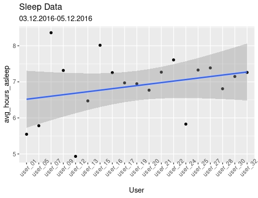
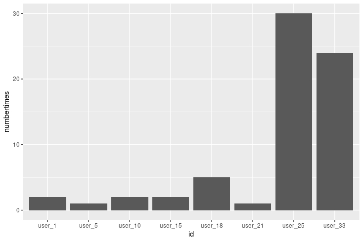
After reviewing these data sets I discovered three major trends. 1) users are getting anywhere between 6 to 8 hours of sleep per night. This is shown in sleep data for twenty users from March 12 to April 12. 2) Within the heart rate and hourly intensities data sets I noticed correlation between hourly intensity and heart rate. These variables are strongly correlated with a correlation coefficient of 0.878. 3) the trends in weightLog_data prove that many users are not consistently logging weight information.

Were you able to answer the business questions? Yes, the trends in non Bellabeat smart device users were discovered, the way in which these trends relate back to Bellabeat customers were defined, and lastly the marketing strategy for the Bellabeat Team was guided.
What story does your data tell? The data story shares how non-Bellabeat smart device users are using their products.
How do your findings relate to your original question? The findings from these dats sets help define how potential Bellabeat customers are using smart devices, this will help direct the marketing strategy for the Bellabeat App.
Who is your audience? What is the best way to communicate with them? My audience is key stakeholders and the best way to communicate with them is through effective presentation.
Can data visualization help you share your findings? Yes, data visualizations are key for displaying results from an analysis.
Is your presentation accessible to your audience? Yes, the presentation is available for stakeholders.

Visualizations and Key Findings

Sleep Patterns

My first analysis is from sleepDay_merged data. I analyzed normal amounts of sleep per user from April to May of 2016.

Sleep Patterns

ggplot(data=sleep_datatwo, aes(x=User,y=avg_hours_asleep, group=1)) +
  geom_point() +
  geom_smooth(formula = y ~ x, method = "lm") +
  theme(axis.text.x = element_text(angle = 45)) +
  ggtitle("Sleep Data",
          subtitle = "03.12.2016-05.12.2016 ")

Heart Rate vs Average Intensity

Next, I visualized the data from user 6 on 2016-04-16 from 7AM to 8PM to show how heart rate varied along with average intensity. The graphs look similar indicating a strong relationship. This relationship is reinforced by a correlation coefficient of 0.878 between heart rate and average intensity.

Heart Rate Plot

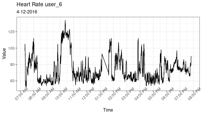
Heart Rate

heartrate_data %>%
  mutate(heartrate_data, Time = as.POSIXct(Time, format = "%m/%d/%Y %I:%M:%OS %p")) %>%
  ggplot(aes(x = Time, y = Value)) +
  geom_line() +
  theme_bw() +
  scale_x_datetime(breaks = "1 hour", date_labels = "%I:%M %p") +
  theme(axis.text.x = element_text(angle = 45)) +
  ggtitle("heart rate user_6",
          subtitle = "4-12-2016")

Average Intensity Plot

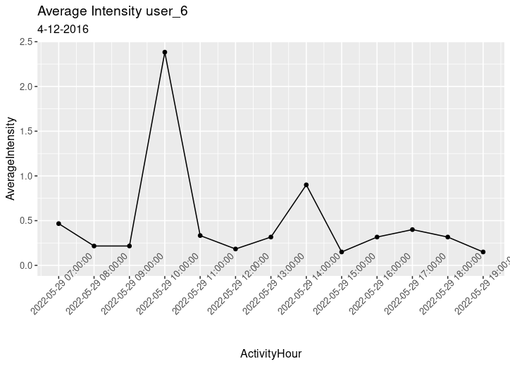
Average Intensity

  ggplot(data=hourlyIntensities_data, aes(x = ActivityHour, y = AverageIntensity)) +
  geom_point() +
  geom_line() +
  theme(axis.text.x = element_text(angle = 45)) + 
  scale_x_datetime(date_breaks = "hour", limits = c(as.POSIXct("2022-05-29 07:00:00"),as.POSIXct("2022-05-29 19:00:00"))) +
  ggtitle("Average Intensity user_6",
          subtitle = "4-12-2016")

Weight Log

My final visualization is indicating a lack of data entry in weight log information. The number of users that logged weight log information is very small with many of them logging less than 5 times for the entire month.

Weight Log plot

ggplot(data = repeated_users, aes(x = id, y = times_used)) +
  geom_bar(stat= 'identity') +
  ggtitle("Weight Log")

Summary Statistics: Sleep Patterns

I decided to create summary statistics for users 5, 13, and 17 in order to analyze specifics of nightly sleep schedules. The users were chosen at random to avoid bias.

filter sleep data for user_5

sleepday_User5 <- select(filter(sleep_data,Id %in% c("1927972279")), c(Id, SleepDay, TotalSleepRecords, TotalMinutesAsleep, TotalTimeInBed, TotalHoursAsleep))

user_13

sleepday_User13 <- filter(sleep_data, Id == 4020332650)

user_17

sleepday_User17 <- filter(sleep_data, Id == 4445114986)

summary statistics:

summary(sleepday_User13$TotalHoursAsleep)

##    Min. 1st Qu.  Median    Mean 3rd Qu.    Max. 
##   3.767   5.717   6.417   6.471   7.667   8.350

summary(sleepday_User17$TotalHoursAsleep)

##    Min. 1st Qu.  Median    Mean 3rd Qu.    Max. 
##   5.367   6.242   7.267   6.971   7.658   8.367

summary(sleepday_User5$TotalHoursAsleep)

##    Min. 1st Qu.  Median    Mean 3rd Qu.    Max. 
##   4.933   5.358   5.783   5.783   6.208   6.633

Step 6 - Act

Guiding questions

What is your final conclusion based on your analysis? The Bellabeat marketing team should focus on the core uses and features that were found in our analysis. Better understanding of these features, development, and marketing will allow the Bellabeat app and other products to grow within the market.
How could your team and business apply your insights? Push marketing strategy in the direction of key uses and features that were found in this report.
What next steps would you or your stakeholders take based on your findings? The next step would be to implement these insights into a productive marketing campaign.
Is there additional data you could use to expand on your findings? The majority of data was taken in the summer months which could create bias, more data based in winter and fall months would be useful.

Insights and Recommendations

To better market the Bellabeat app the marketing team will need to focus on the core uses and strengths that were found in our analysis. Focusing the marketing strategy on the key features which Bellabeat users will use day to day will add the most value to our campaign. In our analysis we see that users are tracking sleep, daily activity, and logging information such as weight. Advertising these features will allow customers to gain an understanding of the product making it more likely for them to consider purchasing the product.

Google Data Analytics Professional Certificate

Capstone #1 - Bellabeat

Brief Introduction

Step 1 - Ask

Business Task

Step 2 - Prepare

Description of Data Sources

Step 3 - Process

Documented Cleaning Process

Import datasets

View datasets

Check for structural errors

Check for irregularities

Cleaning and Filtering

Step 4 - Analyze

Summary of Analysis

Step 5 - Share

Visualizations and Key Findings

Sleep Patterns

Heart Rate vs Average Intensity

Heart Rate

Average Intensity

Weight Log

Summary Statistics: Sleep Patterns

Step 6 - Act

Insights and Recommendations